# Excel formulas
Excel's power is all in the formulas.
Without formulas, Excel is a calculator with a keyboard. With formulas, it becomes a data processing powerhouse that can load, parse, transform, and calculate almost anything.
This guide covers the essential formulas you need to solve 90% of your Excel problems.
## Quick reference
1# Function keys
2
3- Toggle Enter/Edit Mode: `F2`
4- Toggle Reference Modes: `F4`
5
6# Basic operators
7
8- Formula identifier: `=`
9- Define ranges: `:`
10- Separate terms: `,`
11- Group terms: `()`
12- Equality/inequality: `=`, `<>`
13- Comparisons: `>`, `>=`, `<`, `<=`
14- Math: `+`, `-`, `*`, `/`
15- Text quotes: `""`
16- Text joining: `&`
17
18# Essential functions
19
20## Aggregation
21
22- `MIN()` - Find lowest value
23- `MAX()` - Find highest value
24- `COUNT()` - Count numbers
25- `COUNTA()` - Count all items
26- `SUM()` - Add values
27- `AVERAGE()` - Calculate mean
28
29## Conditionals
30
31- `IF()` - If/then logic
32- `COUNTIFS()` - Count with conditions
33- `SUMIFS()` - Sum with conditions
34- `AVERAGEIFS()` - Average with conditions
35
36## Lookup
37
38- `INDEX()` - Find value at position
39- `MATCH()` - Search for position
## Key concepts
### F2: your best friend
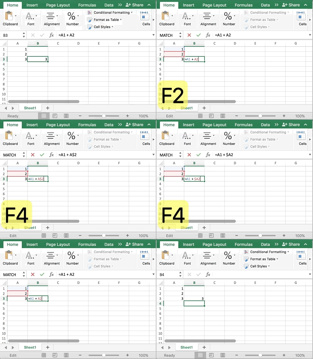
F2 toggles between Enter Mode and Edit Mode. In Enter Mode, arrow keys move between cells. In Edit Mode, arrow keys move within the formula.
Use F2 to edit formulas without touching your mouse. While editing, place your cursor near an operator (+, -, &) and press F2 again to switch back to Enter Mode and add cell references with arrow keys.
### F4: reference locking

F4 cycles through cell reference modes when your cursor touches a cell reference:
- →
$A$1- Lock both row and column - →
A$1- Lock row only - →
$A1- Lock column only - →
A1- No locks
Locked references don't change when you copy formulas to other cells.
## Basic operators
### Formula punctuation
- →
=- Start all formulas with equals sign - →
:- Define ranges (e.g.,A1:B2) - →
,- Separate function arguments - →
()- Group operations and define order
### Comparison Operators
- →
=- Check equality - →
<>- Check inequality - →
>,>=,<,<=- Comparison operators
### Arithmetic Operators
- →
+,-,*,/- Basic math operations
### Text Operators
- →
""- Identify text strings - →
&- Join text together (concatenation)
## Aggregation
### Minimum: MIN()
- →
=MIN(number1, [number2], ...) - →Finds the lowest number in a range. Ignores text.
### Maximum: MAX()
- →
=MAX(number1, [number2], ...) - →Finds the highest number in a range. Ignores text.
### Count numbers: COUNT()
- →
=COUNT(value1, [value2], ...) - →Counts only numeric values in a range.
### Count all items: COUNTA()
- →
=COUNTA(value1, [value2], ...) - →Counts all non-empty cells (numbers and text).
### Sum a range: SUM()
- →
=SUM(number1, [number2], ...) - →Adds all numbers in a range. Ignores text.
### Average a range: AVERAGE()
- →
=AVERAGE(number1, [number2], ...) - →Calculates the mean of numbers in a range. Ignores text.
## Conditionals
### If statements: IF()
- →
=IF(logical test, value if true, [value if false]) - →Returns one value if a condition is true, another if false.
=IF(A1="apple", B1, B2) displays B1 if A1 contains "apple", otherwise B2.
### Count with conditions: COUNTIFS()
- →
=COUNTIFS(criteria range1, criteria1, ...) - →Counts cells meeting multiple criteria. Works in range/criteria pairs.
=COUNTIFS(A:A, TRUE) - Count where column A is TRUE
=COUNTIFS(A:A, TRUE, B:B, 6) - Count where A is TRUE AND B equals 6
### Sum with conditions: SUMIFS()
- →
=SUMIFS(sum range, criteria range1, criteria1, ...) - →Sums cells meeting conditions. First argument is the sum range.
=SUMIFS(A:A, B:B, TRUE, C:C, 6) - Sum column A where B is TRUE and C equals 6
### Average with conditions: AVERAGEIFS()
- →
=AVERAGEIFS(average range, criteria range1, criteria1, ...) - →Averages cells meeting conditions. Works like SUMIFS.
=AVERAGEIFS(1:1, 2:2, TRUE, 3:3, 6) - Average row 1 where row 2 is TRUE and row 3 equals 6
## Matching & Search
### Find value at position: INDEX()
- →
=INDEX(array, row num, [column num]) - →Returns value at specified position in a range.
=INDEX(A:A, 5) → Value in A5
=INDEX(A:D, 1, 3) → Value in C1
### Search for position: MATCH()
- →
=MATCH(lookup value, lookup array, [match type]) - →Finds position of a value in a range. Match types:
- →
0= Exact match (use for text) - →
1= Less than or equal (default) - →
-1= Greater than or equal
- →
=MATCH("some string", A:A, 0) → 4 (if found in A4)
### Why no VLOOKUP?
VLOOKUP() and HLOOKUP() are inefficient, rigid, and prone to breaking silently. Use INDEX() and MATCH() instead for more flexible and reliable lookups.
=INDEX(return_range, MATCH(lookup_value, lookup_range, 0))
Combines INDEX and MATCH to replace VLOOKUP with more flexibility:
- →Handles column insertions/deletions better
- →Faster on large datasets
Example: Look up price for a product
=VLOOKUP("Apple", A:C, 3, FALSE) → Old way
=INDEX(C:C, MATCH("Apple", A:A, 0)) → Better way
The MATCH finds the row, INDEX returns the value from that row.